How to Calculate Luminosity Dominant Wavelength and Excitation Purity

1. Introduction

There are many different systems for analyzing and representing the color of an object perceived by a human observer. For the purposes of unambiguously specifying the color an observer sees when looking through an optical filter at a well- defined light source, we have found the CIE Color Specification System to be the most accurate (for a simple and clear description, see [1]). In this article we briefly describe the method to calculate the three main parameters that fully specify color in this system: luminosity, dominant wavelength, and excitation purity. These terms specifically refer to the definitions in the CIE system given below, but they have analogies in many other systems. A set of more general terms often used to qualitatively describe color are: brightness, hue, and saturation (analogous to luminosity, dominant wavelength, and excitation purity, respectively). These terms (and others) are often used interchangeably. Here we will adhere to the official terms assigned to the CIE system to avoid any ambiguity.

2. Luminosity

Luminosity can be thought of as a measure of the brightness of an object as perceived by a human observer. It is also sometimes called “visible light transmission” (VLT) or “photopic transmission.” It is basically the integrated transmission spectrum of an object over the whole visible spectrum, weighted by the photopic spectral response of a typical human eye. Photopic refers to vision by “cones,” as opposed to scotopic which refers to vision by the more sensitive
but less color-discriminating “rods”. To calculate the luminosity of a filter, simply calculate the area under the transmission spectrum curve weighted by the Photopic Curve V(λ), and divide by (normalize by) the area under the photopic curve. Mathematically, the luminosity L is given by 

where T(λ) is the transmission spectrum of the filter (0 ≤ T ≤ 1). The Photopic Curve V(λ) is available from numerous sources (see, for example, http://cvrl.ioo.ucl.ac.uk/).

The definition in Eq. (1) assumes that spectrally broad, “white” illumination is used (so called “CIE-E” illumination). If a different illuminant is to be used, then the observed spectral response should be weighted by that illuminant as well, such that Eq. (1) becomes

where I(λ) is the spectrum of the illuminant. Typical illuminants in addition to CIE-E (uniform “white” illumination), include: CIE-C (represents average sunlight), CIE-D65 (very close to black-body radiation with a color temperature of 6500K), and CIE-A (represents a typical incandescent lamp).

An example illustrating these calculations is shown in Figure 1. On the left is shown a typical filter transmission spectrum (blue) and the Photopic Curve (red). On the right the product of these two is shown. The luminosity is the area under this product curve divided by the area under the Photopic curve. For this particular example, the luminosity if calculated to be 77%.

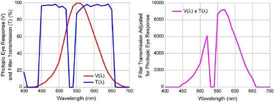
Figure 1: Example illustrating calculation of luminosity for a particular filter transmission spectrum.

3. Dominant Wavelength

In order to calculate dominant wavelength, we must first introduce the identification of a color by its “x-y chromaticity coordinates” as plotted in the Chromaticity Diagram. The diagram enables us to quantitatively graph the hue and saturation of a particular color by its dominant wavelength and excitation purity, respectively.

The first step in calculating the chromaticity coordinates is to compute the “tristimulus values” of a particular filter with a particular illumination. Loosely, the tristimulus values can be thought of as the amount of red, green, and blue in the filter, but the correspondence is not quite that simple. These values are based on the empirically determined CIE Color Matching Functions . Note that we typically use the CIE 1931 2-degree field-of-view standard, as this one is the most well known and widely used. It is useful to note that by definition the   Color Matching Function is identical to the Photopic Curve V(λ), or  . The Color Matching Functions can also be obtained from numerous sources (like http://cvrl.ioo.ucl.ac.uk/). These are illustrated in Figure 2.

The tristimulus values X, Y, and Z are then given by

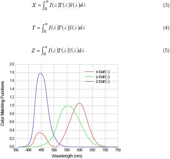
Figure 2: CIE 1931 2-degree field-of-view Color Matching Functions.

As in the calculation of the luminosity, for uniform (CIE-E) illumination, we simply set I(λ) = 1. Note that the Color Matching Functions are typically used in either 5-nm resolution or 1-nm resolution. We find that it is important to use 1-nm resolution for the most accurate determination of color properties of filters, since filters can have very sharp spectral features.  The color, as  determined from the tristimulus values, can now be represented graphically on a two-dimensional graph called the Chromaticity Diagram. The x-y coordinates on this graph are given by

An example of the Chromaticity Diagram is shown in Figure 3. One should be careful not to trust the colors illustrated on the diagram when it is displayed on either a computer screen or a printed hardcopy, as they are not identical to the true colors. On this diagram the x-y coordinates for a number of standard illuminants are shown. Also, one can see that the  pure spectral colors (i.e., truly monochromatic light) trace out a locus of points that looks like a tilted horseshoe, with the violet end of the spectrum on the lower left (near (0,0)), and the red end of the spectrum on the lower right. All other colors lie somewhere inside of this horseshoe-shaped region. Also note that the straight line that connects the violet end of the horseshoe to the red end of the horseshoe represents colors that are a mixture of red and blue (purple), and therefore cannot be realized with a single wavelength of purely monochromatic light. 

The locus of points that define the horseshoe-shaped region are the chromaticity coordinates for spectrally pure colors. These can also be obtained from a number of sources (see, for example, http://cvrl.ioo.ucl.ac.uk/). They are represented graphically in Figure 4.

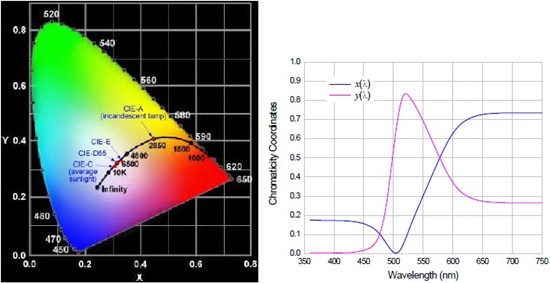
Figure 3: CIE 1931 Chromaticity Diagram.            Figure 4: Coordinates of spectrally pure colors

In order to calculate the dominant wavelength, one simply constructs a line between the chromaticity coordinates of the reference white point on the diagram (for instance, CIE-E, CIEC, etc.) and the chromaticity coordinates of the filter (as computed from Eqs. (6)), and then extrapolates the line from the end that terminates at the filter point. The wavelength associated with the point on the horseshoe-shaped curve at which the extrapolated line intersects is the dominant wavelength. When the line is extrapolated in the other direction (from the end that terminates at the reference white point), the wavelength associated with the point on the horseshoe-shaped curve at which this line intersects is called the “complementary wavelength.” When the line used to locate the dominant wavelength does not intersect the horseshoe-shaped curve at all (i.e., it intersects the straight line that contains the purples near the bottom of the diagram), then the complementary wavelength instead of the dominant wavelength is used to describe the color most accurately, and in this case it is called the “complimentary dominant wavelength.”

Table 1 gives the chromaticity coordinates for some of the more common reference white points, and Figure 5 illustrates the construction of the line to determine the dominant wavelength.

Table 1: Chromaticity coordinates of some common illuminants used as a white reference. Reference White (Illuminant) x coordinate y coordinate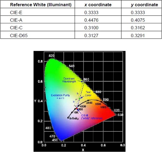

Figure 5: CIE 1931 Chromaticity diagram and illustration of construction of line to determine the dominant wavelength and the excitation purity of a particular test color.

4. Excitation Purity

Once the line is constructed to determine the dominant wavelength, it is very straightforward to calculate the excitation purity of a color that represents the filter transmission. The excitation purity is defined to be the ratio of the length of the line segment that connects the chromaticity coordinates of the reference white point and the color of interest to the length of the line segment that connects the reference white point to the dominant wavelength. These line segments are illustrated in Figure 5. As pointed out above, the excitation purity is a well-defined, quantitative measure of the saturation of a particular color. The larger the excitation purity, the more saturated the color appears, or the more similar the color is to its spectrally pure color at the dominant wavelength. The smaller the excitation purity, the less saturated the color appears, or the more white it is. Pastel colors are very poorly saturated, for example. 

When there is no well-defined dominant wavelength, the excitation purity is still defined as described above, except the denominator should be taken as the length of the line segment between the reference white point and the point at which the dominant wavelength construction line intersects the line that contains the purple colors near the bottom of the diagram.

5. Summary

This article provides a very brief overview of a simple, clear, and unambiguous method for calculating the color an observer sees when looking through an optical filter at a well-defined light source using the CIE 1931 Color Specification System.

References

[1] Daniel Malacara, Color Vision and Colorimetry: Theory and Applications (SPIE Press, Bellingham, 2002).

Author

Turan Erdogan, Ph.D.