Fluorescent Proteins-Theory Applications and Best Practices

First identified in 1962 in sea creatures, fluorescent proteins have proved versatile and extremely useful, as demonstrated by applications they either enable or significantly benefit. The list includes live cell imaging, multicolor gene expression imaging, and flow cytometry, along with an array of biosensors and optical highlighters.

Indeed, fluorescent proteins – or FPs – have turned out to be fundamentally important to science. In 2008, the Nobel Prize in Chemistry was awarded jointly to Osamu Shimomura, Martin Chalfie, and Roger Tsien for their work on the first fluorescent protein, or, in the words of the Nobel Committee, “the discovery and development of the green fluorescent protein, GFP.” 

Where once there was a single fluorescent protein, now there are dozens. They differ in spectral characteristics, environmental sensitivity, photostability, maturation time, and other parameters. In this article, the history and development of FPs is discussed, along with what they are and how they work. Applications of fluorescent proteins are covered, as are considerations for application success. Also covered are some considerations for the optical systems used to view FPs, such as the effects of transmission and other filter spectral characteristics. The conclusion looks at what is needed for future FPs and examines some ongoing development efforts and directions.

Out of the Sea

First identified in the middle of the last century, GFP was originally isolated from the bioluminescent organs of the Aequorea victoria jellyfish. The protein glowed a bright green when exposed to ultraviolet light – hence the name green fluorescent protein. That 1962 discovery was followed by another in 1971 of similar FPs in other sea life. In 1979 Shimomura determined that GFP resembles a soup or soda can in shape and proportion, with an 11-stranded sheet wrapped into a cylinder measuring 42 by 24 Å. The fluorophore sits in the middle of the can.

Other studies have indicated that many fluorescent proteins follow this basic structure, though the fluorophores differ. For example, there is DsRed, a red fluorescent protein from the Discosoma mushroom anemone discovered in 1999. DsRed is the result of ongoing efforts to find far red FPs. The DsRed fluorophore is very similar to the one in GFP, the difference being an extra double bond.

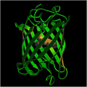
(Photo used with permission from Roger Y. Tsien, Department of Pharmacology, Department of Chemistry & Biochemistry, University of California, San Diego)

The fluorescence in FPs arises after a multistep process which consumes O2 and generates H2O2. This step results in a tightly wound peptide chain triplet ring fluorophore that fluoresces because of the spatial arrangement forced on it by the enclosing structure, the soup can. Since the entire chain is involved, considerable changes can be made to the structure without extinguishing emission. Researchers have taken advantage of this flexibility to produce a whole series of variants and extensions. (See Table 1.)

The list includes new green FPs, with emission maxima around 510 nm, and excitation maxima typically between 475 and 495 nm. An example is enhanced GFP, or EGFP, which has twice the brightness of the “wild type” GFP. There are also blue, cyan, and yellow FPs. In general the blue and cyan have diminished brightness and the yellow has enhanced, as compared to EGFP. For the blue, emission maxima are around 450 nm, while for the cyan and yellow it is 480 and 530, respectively. Excitation maxima run about 40 nm less than the emission maximum for the blue and cyan, while the difference is only about 20 nm for the yellow.

The Fruits of Labor

Complementing these variants are fruit-labeled FPs, ranging from the yellow to orange and into the red. Examples of each are mBanana, mOrange, and mApple, with emission maxima of 553, 562, and 592 nm, respectively. One of the most popular is the aptly named mCherry, with an emission peak at 610 nm and about the same brightness as wild type GFP. Because they emit and absorb at longer and therefore more tissue-benign wavelengths, fruit FPs, which first appeared in 2004, are enabling new applications. 

In addition to finding or creating FPs that span the visible, researchers have also modified these proteins to create more useful versions. One of the primary changes has been in the maturation temperature. Wild type GFPs natively mature at 28° C. By modifying the protein structure, researchers have altered the temperature to a more mammalian friendly 37° C. Unlike standard labeling fluorophores, FPs may be expressed by cells themselves and have been since GFP was first successfully cloned in the early 1990s. To be useful in research the proteins have to mature and achieve fluorescence in a cell-suitable environment.

These maturation changes and modern gene engineering techniques make it possible to transfect organisms with FPs. They were first expressed in 1994 by the microbe E. coli and the worm C. elegans, two species important for biological research. Since then fluorescent proteins have been expressed by a host of organisms, leading to glowing mice and other animals.

Another twist was the creation of photoconvertible fluorescent proteins, which change in response to intense light at an appropriate wavelength. Some transform from a non-fluorescent to a stable fluorescent state. Others switch colors, changing from green to cyan, for example. Also known as photoswitchable or photoactivatable FPs, these creations were developed in the early part of this century.  (See Table 2.)

Putting Fluorescent Proteins to Work

As a result of decades of fluorescent protein development efforts, there are now many applications which are either enabled by or significantly benefit from FPs. One is live cell imaging, one of the first uses of fluorescent proteins. FPs can be fused with other proteins of interest, thereby producing an easily visible indicator in live cells. On a larger scale, the technique can be used to image a given cell category in a tissue made up of various cell types. There are, for instance, transplantation studies done using cells from transgenic mice expressing GFP under the human ubiquitin C promoter.

Live cell imaging can also capture what goes on inside a cell. If the concentration is low enough, then individual proteins can be tracked. For example fluorescent-conjugated actin or tubulin forms fluorescent speckles in either filamentous actin or microtubules. The movement of these speckles can be recorded, resulting in a video of cellular activity. At higher concentrations, statistical methods that analyze intensity can track fluctuations from FPs migrating into and out of a focal volume, thus enabling measurement of protein dynamics and movement.

Since fluorescent proteins may be produced within a cell, they naturally serve as markers for gene expression. When fluorescence is present, the gene is being expressed and vice versa. There is an extension to this idea, made possible by FPs of different colors. If a green FP is fused to one protein of interest and a blue or cyan to another, then the expression of two or more genes can be captured. The idea can be further expanded by using a greater number of different colored FPs. Clearly, this application requires that the fluorescent protein emissions be spectrally distinguishable from one another. It also is best if the FPs can be excited by as few sources as possible, as that makes the setup less complicated.

There are, of course, practical limits in terms of how many fluorescent proteins can be used. The absorption and emission spectra of FP’s tend to be comprised not of fairly narrow, closely spaced peaks but rather of broad spectral tails, leading to substantial overlap of neighboring FP spectra. As a result, high-performance precisely optimized optical filters and careful choice of the light source and detector are required.  Additionally, each FP may respond with different intensity to a given excitation or react differently to a given cellular environment. If quantitative measurements are to be done, such factors have to be accounted for.

There is an application, though, where a simple on-off determination may be sufficient. In flow cytometry, individual cells are tallied as they flow past an interrogation point. The cells of interest are often part of a stream of other cells, which complicates the count. With fluorescent proteins, the task is made much easier, especially if the cells being scanned have little or no native fluorescence at the FP emission wavelength. The cells are transfected with fluorescent proteins, creating specimens that, after the FPs mature, emit a known wavelength in response to a given excitation light. The cells can then pass by a window, be excited by an appropriate light source, fluoresce, and be tallied. This approach can also be used to separate cells of interest from others in a stream.

Sensors and Highlighters

Another set of applications that benefit significantly from FPs involve biosensors. Successful mutagenesis has been carried out to make fluorescent proteins that respond to pH, with emission intensity dropping as acidity climbs. The change arises due to direct interaction with the fluorophore or the enclosing barrel. There can be as much as a 15-fold increase in fluorescence over a 5.5 to 9.5 pH range. Similarly, there are FPs that respond to levels of the important signaling biochemical Ca2+. The sensing comes courtesy of a fused protein and an indirect impact on the fluorophore. There are various incarnations of this approach, with a roughly 10-fold change in fluorescence as concentrations levels change from 10 µm to 1 mm. A third example involves membrane potential sensors, which exhibit only a relatively small change in fluorescence.

Another sensor category involves FRET, or Förster Resonance Energy Transfer. Two fluorophores in close proximity undergo dipole to dipole coupling with one acting as an electron acceptor and the other as a donor. The result is a distance-dependent change in the acceptor fluorescence, but typically only if the distance between the two is measured in nanometers. Thus, FRET can act as a molecular-scale ruler.  

An example of a FRET-based approach can be seen in a sensor to detect phosphorylation, the process by which a phosphate group is added to a protein. Fusing a fluorophore-bearing protein to an FP creates FRET-altered fluorescence, with a given emission characteristic. With phosphorylation of the fused protein, the distance between acceptor and donor changes, modifying emission and allowing detection.

The change in a FRET sensor can be quite large, with the shift a good percentage of the baseline. For example, a FRET-based membrane voltage sensor can have a 40 percent change in output. The list of analytes that can be detected with FRET is large. It includes a host of important biochemicals and changes in those biochemicals.

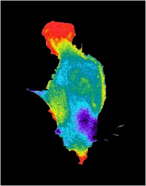
(Photo used with permission from Klaus M. Hahn, Ph.D., Thurman Professor of Pharmacology, University of North Carolina, Chapel Hill)

A final set of applications depends on the ability to switch colors of FPs or to turn them on or off, all in response to intense light. Photoconvertible FPs allow optical highlighting, which conveys several advantages. One important benefit is the ability to control fluorescence over time. An experiment can be run, for example, with fluorescence off until certain conditions are met or a given amount of time has elapsed. In this way, cellular dynamics or tissue reaction in response to specific stimuli can be measured.

Another plus is that these FPs enable imaging previously thought impossible. In classical optics, the diffraction limit is roughly half the wavelength of light. Two objects separated by less than this distance cannot be resolved, which means that features smaller than about 200 nm cannot be seen or studied using visible light and classical optics. With switchable FPs, though, this resolution barrier can be broken. The trick is to switch on the FPs in a succession of groups, creating a series of images made up of sparsely populated point sources. The location of each point source can be determined with a great deal of precision, and the stack of images yields the data needed to reconstruct the entire structure with a resolution far better than the diffraction limit. A ten-fold or better improvement using super-resolution techniques such as Photoactivation Localization Microscopy, or PALM, has already been demonstrated (for more details see the Semrock white paper, “Super-resolution Microscopy”).

Fluorescent Protein Optical Imaging Considerations

FPs have greatly expanded the scientific fluorescence toolbox, thereby enabling new capabilities. At the same time, they also have brought in new aspects to consider. When deciding to use fluorescent proteins in an application, what are the factors that should be taken into account?

It is important to keep in mind that most FP applications involve microscopy, with the wavelengths of interest stretching from the ultraviolet to the infrared. Thus, accessories impacting microscopy imaging are important. For most applications, the emphasis is on the visible. There is, however, an increasing interest in the far red, largely because these photons are less energetic and therefore cause less cellular damage.  (See Table 3.)

Specific applications place different demands. In live cell imaging, for instance, one frequent application is the observation of cellular dynamics. Capturing fast events requires rapid image acquisition, which in turn demands short exposure times. Consequently, the optical system should include high sensitivity detectors and a suitably bright light source, as well as objectives with the right numerical aperture and other characteristics.

The best filter set to use is one optimized for high throughput. Key parameters include very steep spectral edges and high out-of-band blocking, thereby allowing as much of the desired light through while keeping out unwanted stray light. Also, the filters typically need high transmission (%T), which brings important benefits. FPs have to be excited into fluorescence, which means that live cells have to be exposed to excitation light. However, intense excitation light can damage the cells through phototoxicity and can increase the rate of photobleaching. The first damages or kills the cells while the second destroys the FP signal. High %T filters allow more excitation light in and permit better collection efficiency of the emission. As a result, they minimize phototoxicity and photobleaching, and so can enhance live cell imaging.

The fact that live cells are the focus of these applications has other implications for optical components. Typically, cell samples have to be maintained at 37° C, often at a controlled CO2 concentration and humidity. These environmental conditions may be achieved using an enclosure, and any optical filters might be inside the enclosure. In these circumstances, the best choice is likely to be hard-coated filters. They do not degrade or suffer damage as a result of these environmental conditions. Soft-coated filters, on the other hand, can be damaged. In general, in any situation, the reliability of the filters and other optical components is important.

For optical highlighter applications, there are additional considerations. They typically require two distinct excitation bands, one for photoconversion and another for excitation. Both travel over at least some of the same optical path, as does the outgoing emission. Therefore, dichroic beamsplitters and associated filters have to be used. The optics must have wide reflection bands, including reflection in the UV. The latter is needed because photoconversion often requires a UV source.

The challenge is that high energy UV illumination can create cellular damage, so care has to be taken to optimize the illumination intensity. One way to do so is via neutral density filters. Another is to reduce the exposure time. Because of overlapping optical paths, filters in the excitation path need to have good blocking within the passband of any emission wavelengths.

Using optical highlighters to achieve super-resolution places its own demands on optical components. Beating the diffraction limit demands what are effectively multiple passes. Thus, like live cell imaging, this application benefits from high %T filters and the resulting increase in throughput.

In the case of multicolor imaging, there is a need to separate out FP signals. A striking and scientifically important example can be found in the so-called Brainbow mice created by Harvard researchers Jean Livet and Jeff Lichtman in 2007. Now available commercially, these transgenic mice have randomly arranged fluorescent proteins in their neurons. Because the integration sites have multiple copies of the transgene, each neuron may express one of many possible FP combinations and distinct hues. There may be 150+ distinguishable colors, with the expression and resulting color being modified by the use of a promoter.

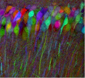
(Photo used with permission from Jeffrey Lichtman, MD, Professor of Molecular and Cellular Biology, Harvard University, Cambridge MA)

In designing the transgenes, the researchers created one with a membrane tether to allow axonal processes to be labeled, another with a nuclear localization signal, and a third that is distributed throughout the cytoplasm. These mice could allow researchers to map the circuits of the brain. However, investigators will have to differentiate between signals in what looks like multicolored abstract art to the naked eye. Thus, there is a need for emission filters with high %T in a passband and little, or no, transmission elsewhere. Furthermore, the filters may need to have a relatively narrow passband. Better performance in these parameters, along with the right characteristics in the detector and microscope, makes the mapping of multicolored images easier.

With regard to other components for multicolor imaging, the objectives need to be color corrected. If they are not, then the signal and image registration for a given set of colors may be adversely impacted. This need for a more uniform – at least well understood – spectral response becomes more important as more colors are used.

A Bright Future

As the Brainbow mice show, new and useful applications of fluorescent proteins continue to appear. These developments are being driven by the ingenuity of researchers and the creation of new FPs with either improved or new capabilities. An examination of current needs reveals areas of possible improvement.

Some involve the creation of FPs with greater photostability. That is, there is a need for fluorescent proteins that generate a more uniform emission over time or space in response to a given excitation. Doing so would allow measurements to be more quantitative and repeatable.

Another ongoing area of development involves red and far red fluorescent proteins for both in vitro and in vivo applications. Such FPs offer multiple advantages. For one thing, the required excitation light would cause less cellular damage than is the case when bluer sources have to be used. For another, the emission can travel further in tissue without being scattered or absorbed. Thus, cellular damage would be minimized and the signal from deep within a cell or tissue maximized, all other things being equal.

If the past is any guide, the development of new fluorescent proteins will lead to new applications, as well as benefiting established ones. The continued progress in what were originally ocean-derived fluorescent proteins represents, in a very real sense, an ongoing sea change in science.

Authors

Hank Hogan is a freelance writer with expertise in science and technology; Prashant Prabhat is Applications Scientist, Nicolas George is Director of Product Marketing, and Turan Erdogan is Co-founder and CTO, all of Semrock, Inc., a Unit of IDEX Corporation.

Table 1: Selected Fluorescent Protein Properties

Source(s): Piston, David W.; Patterson, George H.; Lippencott-Schwartz, Jennifer;  Claxton, Nathan S.; and Davidson, Michael W., Introduction to Fluorescent Proteins, Nikon Microscopy U and Carl Zeiss MicroImaging Online Campus

Lin, Michael Z.; Miyawaki, Atsushi; and Tsien, Roger Y.;  Poster: Fluorescent proteins illuminate cell biology, Nature Reviews, 2010

Table 2: Properties of Selected Optical Highlighters

Source(s): Piston, David W.; Patterson, George H.; Lippencott-Schwartz, Jennifer; Claxton, Nathan S.; and Davidson Michael W., Introduction to Fluorescent Proteins, Nikon Microscopy U

Table 3: Microscope Components Important to Fluorescence Imaging